Category: Physics
-
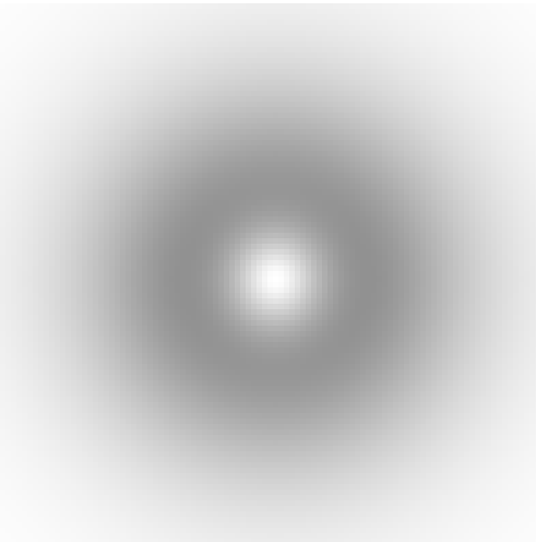
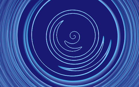
Ring around
This is another shot from the quantum superposition viewer. Â It’s neat as op art, but I’m still trying to fully grasp the realization I made that this represents an unchanging distribution of a unit of rotational motion. Â The state is fixed, but it contains within it an orbiting particle. Related Images:
-
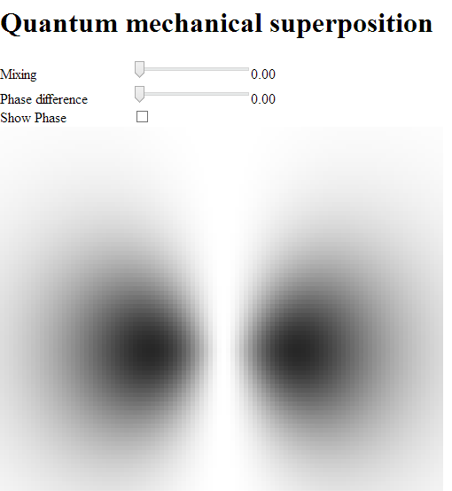
Current project
I’m playing around with quantum mechanical superposition and hydrogen wave functions again.  This time with really simple 2 dimensional renderings.  I’ve been trying to get a grip on some of the basic principles and this is what I’ve got up so far. I’m learning a lot, and there is quite a bit to be gained from playing…
-
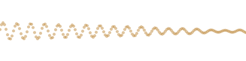
All things must pass
This article reminded me of one of the strange features of the standard wave equation from basic physics. Â The wave equation describes an infinitely long vibrating string. Â Like point masses from Newtonian physics each bit of string has a position and velocity. Â If you know the position and velocity of the entire string at one…
-

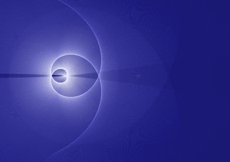
Something different about this one
Continuing on the theme of central forces. This is an initial image of the next guy I’m looking at. This one is pretty similar to the others I’ve done except for that empty circle in the center. Related Images:
-
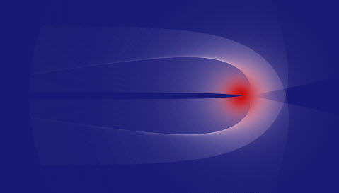
Gravitational slingshots
In my last few posts, I’ve been trying to characterize different potentials through the shapes of their orbits (gravitational, harmonic, lorentz). In the middle of it, I came across a post on bad astronomy about gravitational slingshots. I figured it would be a perfect opportunity to use these images to show the effect in a…
-
A less idealized central force
This is the 3rd in a series that started with the gravitational potential, and then the harmonic. While those are the two biggies, what we are looking at next behaves more like something you would see in real life, and doesn’t have solutions that can be written down with simple formulas. For this entry in…
-
Central force images #2
This is the second in a series profiling the solutions to common central force fields from physics. Check out the the first one on the Newtonian gravitational force field. These are even more plain than the gravitational well. That’s because these are for the harmonic potential. One of the things that distinguishes this potential is…
-
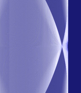
These aren’t all that pretty
Any guesses as to what these are? Rather than focus on chaotic dynamics I wanted to see how I could explore the differences between the classical central forces. This one is newtonian gravity. Related Images:
-
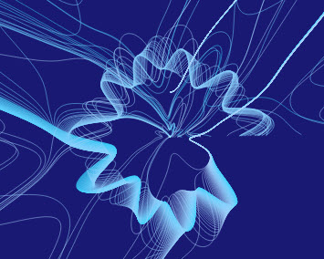
Islands of stability
This time I mapped the pendulum angle and time onto the surface of a cone to create a tunnel effect. For the parameter space I’m looking at, you can really see how the paths will converge for a while and then suddenly diverge wildly. Related Images:
-
Sensitive dependence on initial conditions
This next demo highlights the butterfly effect. These curves show the same pendulum as before, this version has the time axis wrapped around the center of the screen and the exponential of the angle as the radius. All the pendulums start at a very similar initial position and for some driving functions they diverge wildly…