The chaos game
Throw a point at random through the maps, plot where it lands, and a theorem guarantees the attractor draws itself. The renderer is trivial. The tone map is where the work is.
The chaos game is the algorithm that shouldn’t work. You take a point, pick one of the maps at random, apply it, plot the point, and repeat a few hundred thousand times. That’s it. There is no recursion, no subdivision, no representation of the attractor anywhere in the program.
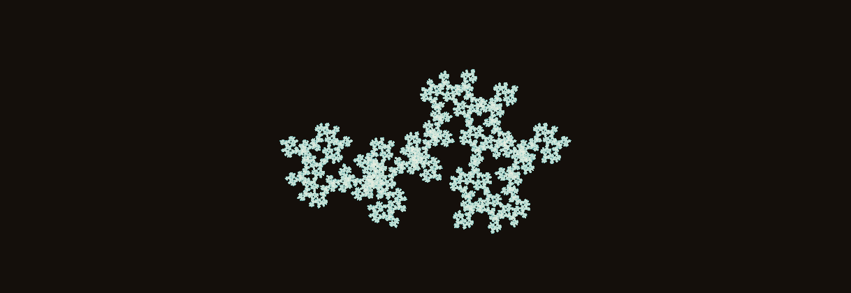
Chaos CPU. A single point, thrown through three maps two hundred thousand times a frame.
It works because of what the maps are. Every is a contraction, so the attractor satisfies : once you are on the set, no map can take you off it. And because , applying maps at random walks you around the whole of and nowhere else. Start off the set and the contraction pulls you onto it geometrically fast — after a couple of dozen maps the error is smaller than a pixel, which is why the renderer runs sixty throwaway iterations at startup before it begins plotting anything.
What makes it fill the set rather than wander a corner of it is Elton’s ergodic theorem. Choose map with probability , and the fraction of time the orbit spends in any region converges to a fixed measure supported on the whole attractor. You get the shape for free from the contraction; you get the coverage from the ergodic theorem. Weighting by — how much area each map keeps — is what keeps the sampling roughly even, since a map that shrinks hard needs proportionally fewer visits to fill its image.
Picking a map from the cumulative probabilities is a binary search, which is the only clever line in the loop:
const pick = (r) => {
  const probs = compiled.cumProb
  let lo = 0, hi = probs.length - 1
  while (lo < hi) {
    const mid = (lo + hi) >> 1
    if (r < probs[mid]) hi = mid
    else lo = mid + 1
  }
  return lo
}
Everything else is a multiply-add and an array increment. The renderer does not accumulate colour; it accumulates a Uint32Array of hit counts, one per pixel. Turning that density buffer into an image is the entire remaining problem, and it is much harder than the iteration.
The tone map is the algorithm
A density buffer is not a picture. Some pixels near the dense core of the attractor get hit thousands of times more often than pixels out on the thin filaments, and a linear map from count to brightness throws all of that away — the core saturates to white, the filaments round to black, and you see a blob.
The obvious fix is an exposure curve, , which is what this renderer used for a long time. It has a fatal property that only shows up once you leave it running. The density buffer at rest accumulates without bound: every frame adds another 220,000 samples to the same counts. So grows without limit, everywhere the set is lit, and the whole attractor converges to one flat cream colour. I measured it: 96.6% of lit pixels were clipped to the identical value. Lowering does not fix this. It delays it.
The exposure constant is the wrong knob because there is no correct value for it — the right value depends on how long you have been watching. What is actually stable is the ratio between densities, so the settled render normalizes against the running maximum on a log scale:
with . The logarithm compresses the enormous dynamic range between core and filament; dividing by the running peak makes the result independent of elapsed time. After that change, clipping fell from 96.6% of lit pixels to 0.1%, and the density gradient inside the attractor becomes visible for the first time.
Dragging is a different problem
There is a second regime, and it wants the opposite of everything above.
While you are dragging a control point the maps change every frame, which means the density buffer is invalidated and cleared every frame. Nothing accumulates. A single frame’s samples have to carry the entire image on their own, and there are far fewer of them because the frame has to land inside a pointer-move.
So the trade inverts. At rest: many samples, each contributing very little opacity, accumulating over seconds into a smooth gradient. While dragging: fewer samples — 70,000 instead of 220,000, because the frame has to be cheap — each composited at high opacity so the attractor stays legible under your hand. It comes out darker and coarser, and that is correct. You are looking at the shape, not the shading.
Mid-drag, 95.9% of lit pixels sit at the top of the ramp. On release, that drops to 0.0% and the gradient blooms back in over a second or two. Two numbers, exactly inverted, which is a satisfying way for a renderer to behave.
The same game on the GPU

Chaos WebGL2. Sixty-five thousand points, all walking at once.
The GPU version does not run one orbit. It runs 65,536 of them in parallel, holding the positions in a floating-point texture, stepping every point through a randomly chosen map in a vertex shader, and writing the new positions back out through transform feedback. The plotted points are composited additively, so the framebuffer is the density buffer, accumulated in hardware.
The drag trade shows up here too, in the only currency additive blending understands: source alpha. At rest each point contributes and three passes run per frame. While dragging, one pass runs and . Same idea, different spelling.
There is no tone map on the GPU path, because there is no readback to normalize against — which means it will still saturate on a long rest where the CPU path holds. That one is unfinished, and I would rather say so than pretend the two agree.
On the default maps the CPU path lights about 28,700 pixels and the GPU path about 26,100 — a few percent apart, which is what you’d expect from two different samplers and two different composites landing on one set. That figure is the closest thing this project has to ground truth, and in three ways to lose a fractal it is what caught two other renderers drawing something else entirely.