Tag: diffeq
-
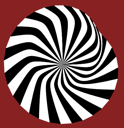
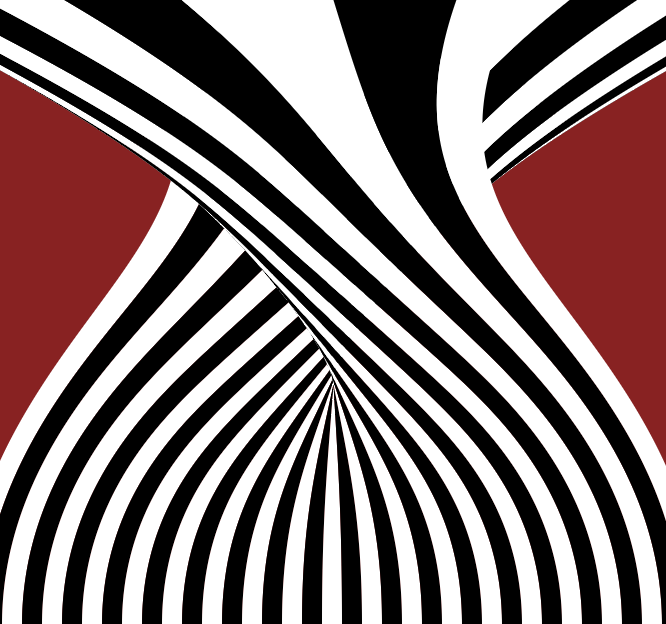
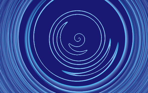
Askew Op Art Disk – Where’d the symmetry go?
The same equations were used to generate this image as well.  The only difference is the starting point.  Instead of expanding from the center of the distortion field, the starting point is displaced a little bit towards the bottom.  This highlights a number of different things. First while the equations are symmetric, the resulting image is…
-
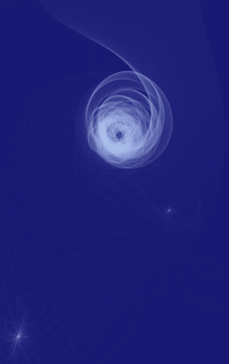
Circling back to a dead end.
These renderings never really went anywhere. They show chaotic orbits around 3 fixed attractive potentials while varying a uniform magnetic field. There are some lovely sweeps and folds as the chaos unfolds. I also like the glowing effect as the orbits get tightly wrapped around the centers of attraction. There wasn’t much to this other…
-
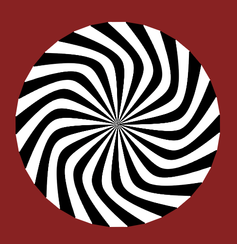
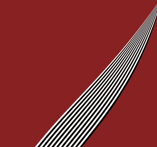
Simple Op Art disk
This is what you get if you take the parallel stream from the rest of the series and replace them with a circular spray from the center of the distortion. Â Everything gets bent uniformly when it hits the ring. Â Moving to second order equations gives you the freedom to have multiple directions from a single…
-
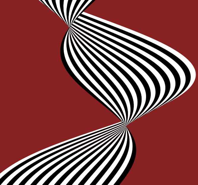
Twist #3
Double twist and wrap. Â While the last image was on the lackluster side, this one has everything turned up to 11. Â There is a strong deflection as the particles pass through the first peak and then they are swung back again as they exit the ring on the other side. Â An important thing to notice…
-
Twist #2
While this isn’t as dramatic as some of the other images, it shows what happens as either the velocity of the particles increases or the strength of the distortion diminishes. Â Instead of dramatic changes, things just tighten up a little bit and bend. Related Images:
-
Simple twist
This shows the distortion in flow from a simple annular distortion. Â It’s part of a series that started with “distortion” and “a single twist and spray“ Related Images:
-
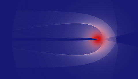
Gravitational slingshots
In my last few posts, I’ve been trying to characterize different potentials through the shapes of their orbits (gravitational, harmonic, lorentz). In the middle of it, I came across a post on bad astronomy about gravitational slingshots. I figured it would be a perfect opportunity to use these images to show the effect in a…
-
Central force images #2
This is the second in a series profiling the solutions to common central force fields from physics. Check out the the first one on the Newtonian gravitational force field. These are even more plain than the gravitational well. That’s because these are for the harmonic potential. One of the things that distinguishes this potential is…
-
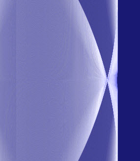
Islands of stability
This time I mapped the pendulum angle and time onto the surface of a cone to create a tunnel effect. For the parameter space I’m looking at, you can really see how the paths will converge for a while and then suddenly diverge wildly. Related Images: