Tag: quantum mechanics
-
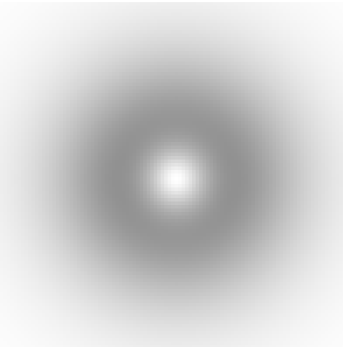
Ring around
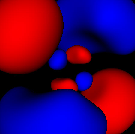
This is another shot from the quantum superposition viewer. Â It’s neat as op art, but I’m still trying to fully grasp the realization I made that this represents an unchanging distribution of a unit of rotational motion. Â The state is fixed, but it contains within it an orbiting particle. Related Images:
-
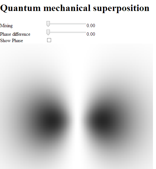
Current project
I’m playing around with quantum mechanical superposition and hydrogen wave functions again.  This time with really simple 2 dimensional renderings.  I’ve been trying to get a grip on some of the basic principles and this is what I’ve got up so far. I’m learning a lot, and there is quite a bit to be gained from playing…
-

All things must pass
This article reminded me of one of the strange features of the standard wave equation from basic physics. Â The wave equation describes an infinitely long vibrating string. Â Like point masses from Newtonian physics each bit of string has a position and velocity. Â If you know the position and velocity of the entire string at one…
-
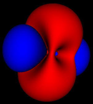
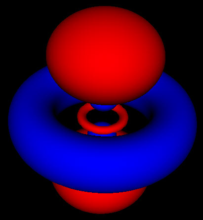
I never knew it looked like that
These are all images of the same electron orbital. The doughnut or torus shows the electron rotating around the central point in the orbital plane. In the standard terminology this has principal quantum number 2, which represents the energy level of the electron. The azimuthal quantum number is 1. This represents how much of…
-
Release often
The atomic orbital viewer is now on it’s third release. The first one was just the basic blurry transparent renderer, using just the rotating basis from the standard derivation from undergraduate physics classes. The second release added an option to view standing wave functions instead of the rotating as the standing wave functions are the…
-

Static images
I’ve added static images of the atomic orbitals from the app. http://curvatureofthemind.com/images/atomic/ Related Images:
-
Electron sausages?
I just paused writing an article where I tried to give a quick overview of quantum mechanics. Ha Ha It ended up being a few paragraphs, a few images, and a crap load of links to Wikipedia. I’m not going to write anything like that anytime soon, and definitely not in a single blog post.…